Solving Black-Scholes

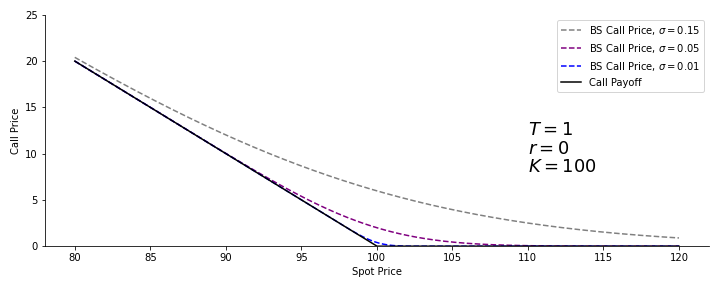
In this section we will obtain an analytical formula for the price of a call option by solving the Black-Scholes equation. It is interesting to note that a change of variables of the Black-Scholes equation yields the differential equation for heat flow in one dimension. Since the heat flow equation is analytically solvable, this is precisely what we will do. So, we begin with $$ \frac{\partial C}{\partial t} + \frac{1}{2}\sigma^2 S^2 \frac{\partial^2 C}{\partial S^2} + rS \frac{\partial C}{\partial S} - rC = 0. $$ The first change of variables is $Z = \log S$. We use the chain rule $$ \frac{\partial}{\partial S} = \frac{\partial Z}{\partial S} \frac{\partial}{\partial Z} = \frac{1}{S} \frac{\partial}{\partial Z} $$ $$ \frac{\partial^2}{\partial S^2} = \left( \frac{\partial Z}{\partial S} \right)^2 \frac{\partial^2}{\partial Z^2} + \frac{\partial^2 Z}{ \partial S^2} \frac{\partial }{\partial Z} = \frac{1}{S^2} \left( \frac{\partial^2}{\partial Z^2} - \frac{\partial}{\partial Z} \right) $$ and substitute the results into the Black-Scholes Equation to get $$ \frac{\partial C}{\partial t} + \frac{1}{2}\sigma^2 \frac{\partial^2 C}{\partial Z^2} + \left(r - \frac{1}{2} \sigma^2 \right) \frac{\partial C}{\partial Z} - rC = 0. $$ Now let's change the time variable to consider the time until expiry: $\tau = T-t$. This only changes the sign of the time-derivative term. $$ -\frac{\partial C}{\partial \tau} + \frac{1}{2}\sigma^2 \frac{\partial^2 C}{\partial Z^2} + \left(r - \frac{1}{2} \sigma^2 \right) \frac{\partial C}{\partial Z} - rC = 0. $$ Next, we introduce a change of variables to take into account the risk-free rate: $C = e^{-r\tau}D$. Substituting this into the equation gives $$ -\frac{\partial D}{\partial \tau} + \left( r - \frac{1}{2}\sigma^2 \right) \frac{\partial D}{\partial Z} + \frac{1}{2}\sigma^2 \frac{\partial^2 D}{\partial Z^2} = 0. $$ What remains now is to get rid of the first-order derivative, which we can do with the substitution $$ y = Z - \left( r - \frac{1}{2} \sigma^2 \right)\tau, \hspace{2mm} s=\tau $$ $$ \frac{\partial}{\partial Z} = \frac{\partial y}{\partial Z} \frac{\partial}{\partial y} + \frac{\partial s}{\partial Z} \frac{\partial}{\partial s} = \frac{\partial}{\partial y} $$ $$ \frac{\partial}{\partial \tau} = \frac{\partial y}{\partial \tau} \frac{\partial}{\partial y} + \frac{\partial s}{\partial \tau} \frac{\partial}{\partial s} = \left( r - \frac{1}{2} \sigma^2 \right) \frac{\partial}{\partial y} + \frac{\partial}{\partial s} $$ Substituting these expressions into the differential equations cancels out the first-order term, leaving $$ \frac{1}{2} \sigma^2 \frac{\partial^2 D}{\partial y^2} = \frac{\partial D}{\partial s}. $$ This equation is the famous heat diffusion equation, and we can obtain the solution by substituting in an appropriate solution and solving according to the boundary conditions. Using change of variables to produce the heat diffusion equation from Black-Scholes is known to be asked in interviews. Solving this equation is quite involved and it is highly unlikely you will be asked to go through it in an interview. Therefore, we will skip the details to instead focus on the solution. The solution for the payoff of a call option is $$ C(S, t) = SN(d_1) - K e^{-r(\tau)} N(d_2) $$ $N$ indicates the cumulative distribution for a standard normal distribution, and where $d_1$ and $d_2$ are $$ d_1 = \frac{\log(S/K) + (r + \frac{1}{2}\sigma^2)\tau}{\sigma \sqrt{\tau}} $$ $$ d_2 = \frac{\log(S/K) + (r - \frac{1}{2}\sigma^2)(\tau)}{\sigma \sqrt{\tau}} $$ These formulae look intimidating, however notice that the only difference between $d_1$ and $d_2$ is a single minus sign. It is worth memorising this formula. Let's now use put-call parity to derive the Black-Scholes price for a put option. $$ C - P = S - Ke^{-r(\tau)} $$ $$ P = C - S + Ke^{-r(\tau)} $$ $$ P = S N(d_1) - Ke^{-r(\tau)} N(d_2) - S + Ke^{-r(\tau)} $$ $$ P = -S \left( 1 - N(d_1) \right) + Ke^{-r(\tau)} \left( 1 - N(d_2) \right) $$ $$ P = -S N(-d_1) + Ke^{-r(\tau)} N(-d_2). $$ The fact that the Black-Scholes equation can be expressed as a heat diffusion equation gives us a useful interpretation of the option value before expiry. As we go backwards in time, the option value is the final option payoff diffused along the spot values, similarly to how heat diffuses through a wire as time goes forward. A plot displaying some option prices as a function of time to expiry, $\tau$, is shown below.

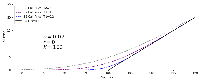
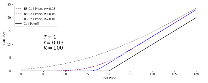
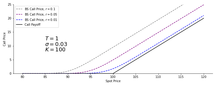
The Black-Scholes prices for a call option

×

❮

❯

We see that call options become more valuable as the time to expiry increases, with the option price converging to the option payoff as the time to expiry approaches zero. To see this, consider that as the time to expiry increases, the variance of the terminal distribution of potential stock values increases as there is more time for the stock to reach higher (or indeed, lower values). As a result, there is more of the probability distribution at higher values above the strike price. Call options become more valuable as volatility increases for the same reason. The variance of the probability distribution of the asset at expiry increases as volatility increases. Call options also increase in value as the risk-free rate increases. This makes sense, since the mean of the terminal probability distribution of the asset is given by $\text{E}[S_T] = S_0 e^{rT}$. Increasing the risk-free rate therefore shifts the probability distribution to larger values, increasing the probability that the option expires in the money.

A useful approximation for the value of an at-the-money call option is $$ C(S, t) \approx 0.4 S \sigma \sqrt{\tau}. $$ This result comes from the fact that if an option is at the money, $S = Ke^{-r\tau}$, and by substituting in this expression we can rewrite the Black-Scholes equation as $$ C(S, t) = S \cdot \left\{ N\left(\frac{1}{2}\sigma\sqrt{\tau}\right) - N \left( -\frac{1}{2}\sigma\sqrt{\tau} \right) \right\}. $$ Taylor expanding this expression will cause the zeroth-order and second-order terms to cancel each other out, leaving the first order term and higher order negligible terms. $$ C(S,t) \approx S N'(0) \sigma \sqrt{\tau}. $$ $N'(0)$ is just the value at $x=0$ of standard Gaussian distribution $n(0) = \frac{1}{\sqrt{2\pi}} \approx 0.4$. Plugging this in gives us the result. It is definitely worth remembering this formula, since it provides you the ability to calculate the value of at-the-money call options in your head. Such questions are often asked in technical interviews.

The put option price behaves similarly as a function of expiry. If the risk-free rate is zero, then the put price increases as a function of time to expiry. Above a threshold value of the risk-free rate however, increasing time to expiry will decrease the price of the option. The risk-free rate increases the mean of the terminal probability distribution of the asset. Since the Black-Scholes formula only prices European options, then it is possible for the put price to be lower than the intrinsic value of the option as it is expected that the stock price will increase according to the risk-free rate by the time the option expires.

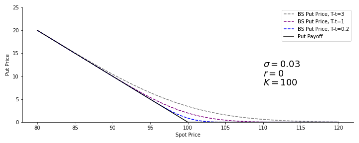
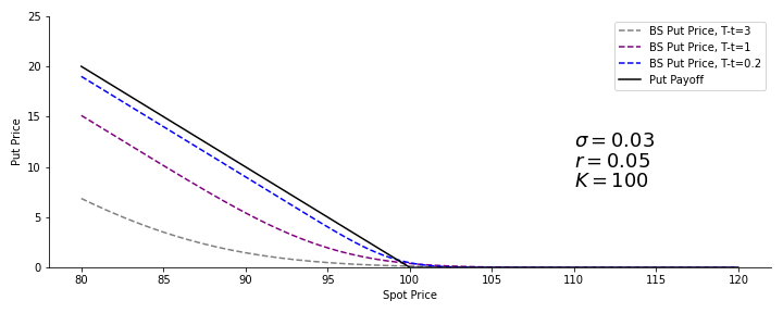
The Black-Scholes prices for a put option

×

❮

❯

Like call options, put options also increase in value according to volatility. These relations we have described between the option price and various parameters are quantified by metrics known as Greeks, and we will cover them in the next section.