Normal Models

We saw in the section on Random Processes that we can consider Brownian motion as the cumulative sum of $n$ samples of a random variable $X_k$, where $$ X_{k} = \begin{cases} \sqrt{\Delta} \hspace{4mm} \text{with probability 0.5}\\ - \sqrt{\Delta} \hspace{2mm} \text{with probability 0.5}. \end{cases} $$ We can draw a connection between an up-move or down-move at a time step $k$, and the outcome of the random variable $X_k$. Let's construct a random process $S_t$ such that $$ S_t = S_0 + \sum_{k=0}^N X_k. $$ Suppose that there are $u$ up-moves in $N$ steps, then $$ S_t = S_0 + u\sqrt{\Delta} - (N - u)\sqrt{\Delta} = S_0 + (2u - N)\sqrt{\Delta}. $$ We can see that this is equivalent to the binomial tree with $\sqrt{\Delta} = q$. We saw in the section on Random Processes that if we let $N$ go to $\infty$, the quantity $$ \sum_{k=0}^N X_k $$ is a Brownian motion with variance equal to the time $t$. The probability distribution for a Brownian motion, which begins at $t=0$ with some initial value $S_0$ and terminates at $t=T$, is a normal distribution with mean $S_0$ and variance $T$. $$ \lim_{N \rightarrow \infty} S_0 + \sum_{k=0}^N X_k = S_0 + \sqrt{T} \: N(0, 1) $$ Another way to understand the relationship between binomial trees and the normal model is to recognise that the probability mass function of the binomial distribution, $f(k,n,p)$, approaches a normal distribution for large $n$ and provided that $p$ is not too close to zero or one. $$ f(k,n,p) \sim N(np, np(1-p)). $$ Since we have established that $p=0.5$, this approximation works perfectly for our purposes. All that remains to obtain our model is to map the number of time steps, $n$, to time $t$. Assets differ in how much they vary in price over time. Some assets are extremely stable, whereas assets like cryptocurrencies are known for having extremely high variability. However, we see that in our model that the variance of the asset price in the future is the same for all assets and is equal to $t$. We call the tendency for asset prices to have different variances in time {\bf volatility}. Assets with higher variance are more volatile and stable assets are less volatile. Volatility is an extremely important concept in finance and we have a section dedicated to it later on in the course. So, an issue with this stock model is that it does not take the volatility of the stock into account. To incorporate volatility, we can introduce a parameter into the variance of the normal distribution. Let us denote this parameter $\sigma$ $$ S_t = S_0 + \sigma \sqrt{T} \: N(0, 1). $$ If $\sigma$ is higher, then the normal distribution of possible future asset prices has larger variance and vice versa. The model now includes an asset-specific parameter. We will see how to calculate this parameter for an asset in the volatility section. A diagram illustrating this model is displayed below. Here, we sample the normal model many times to produce a histogram of the terminal probability distribution, and on the histogram we overlay the normal distribution.

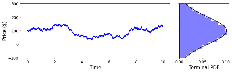
A diagram illustrating the normal model

×

❮

❯

How can we price an option using the normal model? Since the stock values are now continuous, we need to integrate over the probability distribution multiplied by the payoff. Let us define a payoff function, $g(S)$. For a call option the payoff function is $$ g(S) = (S - K)_+. $$ and to calculate the payoff of an option we must calculate $$ \text{E}[\text{Payoff}] = \frac{1}{\sqrt{2 \pi}} \int_{-\infty}^{\infty} g(S_0 + \sigma \sqrt{T} x) \cdot e^{-\frac{x^2}{2}} \text{d}x $$ As it turns out, the normal model is rarely used in practice. The first problem with the normal model is that the normal distribution is nonzero from $-\infty$ to $\infty$. A consequence of this is that the stock can take on negative values, which of course is impossible. Secondly, it is most natural to consider percentage moves of a stock rather than absolute moves. For example, consider two stocks $A$ and $B$. Stock $A$ is €10 and stock $B$ is €1000. Clearly, the stock $A$ increasing in value by €1 is much more significant than stock $B$ increasing in value by €1. However, stock $A$ increasing by 1% is similar in significance to stock $B$ going up 1%. Performance in finance is quantified by relative returns and not absolute returns. So, we want to consider price movements in a relative way rather than an absolute way. An elegant way to implement a model that fits our new requirements is to model the logarithm of the stock as a Brownian motion. Let's consider the stock model $$ \log S_T = \log S_0 + \sigma \sqrt{T} \: N(0, 1). $$ We see that $S_T$ is distributed as $$ S_T = S_0 e^{\sigma \sqrt{T} \: N(0,1)}. $$

We see from the calculation above that the variance of the distribution introduces some drift, so that the mean of the lognormal distribution changes in time. If we impose the condition that the expected value of the asset is constant over time, that is $$ \text{E}[S_t] = S_0, $$ then we must introduce an additional term into the equation. $$ \log S_T = -\frac{\sigma^2}{2} T + \log S_0 + \sigma \sqrt{T} \: N(0, 1). $$ This additional term is known as the Ito correction, and comes up frequently in financial models. Now, $S_T$ is distributed as $$ S_T = S_0 e^{-\frac{\sigma^2}{2} T + \sigma \sqrt{T} \: N(0,1)}. $$ A diagram of this process is shown below.

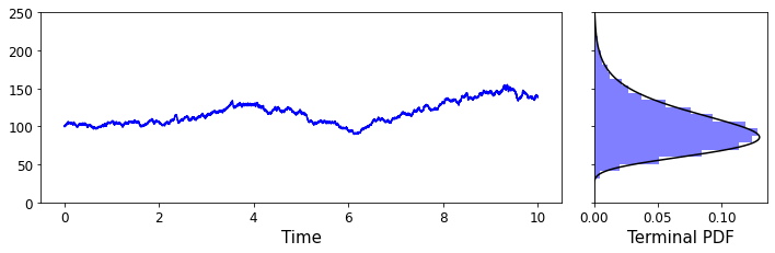
A diagram illustrating the lognormal model

×

❮

❯

This model is the lognormal model without interest rates. Same as before, we calculate an option with payoff function $g(S)$ as $$ \text{E}[\text{Payoff}] = \text{E}[g(S_T)] = \text{E}[g(S_0 e^{-\frac{\sigma^2}{2} T + \sigma \sqrt{T} \: N(0,1)})]. $$ For a call option struck at $K$, this evaluates to $$ \text{E}[\text{Payoff}] = \frac{1}{\sqrt{2 \pi}} \int_{-\infty}^{\infty} (S_0 e^{-\frac{\sigma^2}{2} T + \sigma \sqrt{T} x} -K)_+ \cdot e^{-\frac{x^2}{2}} \text{d}x. $$ In the next section, we will develop the models further by incorporating interest rates.