Options Pricing
The Greeks
In this section we will introduce the Greeks, a set of metrics used to describe the behaviour of option prices under a change of one of their parameters. They are essential tools used for managing risk in options trading and for understanding the various factors that affect the price of an option.
The Greeks are a set of measures that describe how the price of an option changes in response to change of a certain variable. Each Greek is a partial derivative of an option price with respect to the given variable, and are labelled by a Greek letter. Let's outline the commonly used Greeks and then discuss some of their properties.
Delta ($\Delta$)
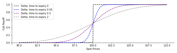
Delta measures the rate of change of the option's price with respect to changes in the underlying asset's price, $\Delta = \frac{\partial C}{\partial S}$. For a call option, delta is between 0 and 1, and for a put option, it's between -1 and 0.
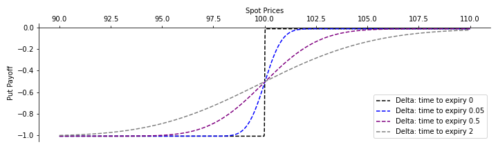
Likewise, the delta of a put option evaluates to $$ \Delta_{\text{put}} = -N(-d_1). $$
In the same way that an option price far from expiry is a smoothed function of the option payoff at expiry, the delta far from expiry is smeared out form of the delta at expiry. As the option approaches expiry, the delta approaches the derivative of the final payoff of an option. Remember that the call option payoff is zero until the spot price is above the strike, after which it increases with a derivative of 1. The delta at option expiry is therefore a Heaviside step function $H(S-K)$, defined as $$ \Delta_{\text{call}}(t=T) = H(S-K)= \begin{cases} 0& \text{if } S-K<0\\ 1& \text{if } S-K \geq 0.\\ \end{cases} $$ Likewise, for a put option, the delta approaches the derivative of the put option at expiry, which is -1 when the put option is in the money, and 0 otherwise. The functional form of this is a negative Heaviside step function. $$ \Delta_{\text{put}}(t=T) = -H(K-S)= \begin{cases} 0& \text{if } K-S<0\\ -1& \text{if } K-S \geq 0.\\ \end{cases} $$
Delta of a call and a put option
Delta is perhaps the most important Greek. It is of foundational importance for hedging. We saw when covering binomial trees that we can obtain some portfolio consisting of options and the underlying asset to make the portfolio invariant in value regardless of how price changes in the future. We denoted the ratio $\Delta$, and in actuality the ratio required to have a portfolio invariant in time is the Greek $\Delta$. A crucial fact is that $\Delta$ changes as the price of the underlying asset changes, and one of the core assumptions of the derivation of the Black-Scholes equation is that we can dynamically hedge the portfolio with no transaction costs. This means that if we hold an option, we assume that we can buy or sell the underlying asset for no cost to change the quantity $\Delta$ so that it is always equal to $\frac{\partial C}{\partial S}$. Provided that we can do this, the total value of the portfolio is invariant to small changes of the underlying asset value price. When the portfolio is invariant in this way, it is described as {\it delta-hedged} or {\it delta-neutral}. In practice, when traders delta hedge, they often impose a threshold where if the value of the underlying asset price changes by some value greater than the threshold, then they rebalance - buying or selling some quantity of the underlying so that the new delta is equal to the current value of $\frac{\partial C}{\partial S}$. $\Delta$ is also used as a proxy for the probability of an option expiring in-the-money. This is only approximately correct, since the probability of a call option expiring in the money is given by $$ P(S_T \geq K) = N(d_2) $$ and for a put option it is given by $$ P(S_T \leq K) = N(-d_2) $$ which are slightly different to the formulae for $\Delta$. It is worth proving the above relations for yourself. As the volatility $\sigma$ approaches zero, $\Delta$ approaches the probability of the option expiring in the money. Therefore this proxy is most valid in lower volatility regimes.
Gamma ($\Gamma$)
While $\Delta$ measures the sensitivity of the option price relative to the price of the underlying, $\Gamma$ measures the sensitivity of the $\Delta$ to the price of the underlying. \noindent Show that $$ \Gamma_{\text{call}} = \Gamma_{\text{put}} = \frac{n(d_1)}{S \sigma \sqrt{\tau}} $$ We saw that $\Delta_{\text{call}} = N(d_1)$ and $\Delta_{\text{put}} = -N(-d_1)$. Therefore, $$ \Gamma_{\text{call}} = n(d_1) \frac{\partial d_1}{\partial S} $$ and $$ \Gamma_{\text{put}} = -n(-d_1) \frac{\partial (-d_1)}{\partial S} = n(-d_1) \frac{\partial d_1}{\partial S}. $$ Given that $n(x) = \frac{1}{\sqrt{2 \pi}} e^{-\frac{x^2}{2}}$, then $n(d_1) = n(-d_1)$. What remains is to compute the partial derivative $\frac{\partial d_1}{\partial S}$. Recall that $\log(\frac{S}{K}) = \log(S) - \log(K)$, so we only need to take the partial derivative of $\log(S)$. $$ \frac{\partial d_1}{\partial S} = \frac{1}{\sigma \sqrt{\tau}} \frac{\partial \log (S)}{\partial S} = \frac{1}{S \sigma \sqrt{\tau}}. $$ Therefore, $$ \Gamma_{\text{call}} = \Gamma_{\text{put}} = \frac{n(d_1)}{S \sigma \sqrt{\tau}}. $$
Gamma of an option
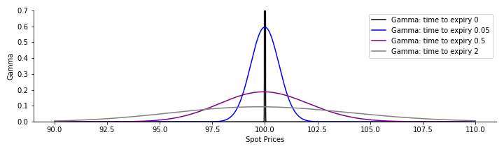
Gamma is typically largest when the spot price is close to the strike price. At the strike price, the option price function has the largest curvature. If the spot price is far from the strike price, that is if the option is deeply in-the money or out-of-the-money, $\Gamma$ is small and $\Delta$ is not particularly sensitive to changes in the spot price. Away from the option expiry, $\Gamma$ looks similar to a normal distribution. As the option approaches expiry, the variance of the function decreases until at expiry $\Gamma$ is equal to a Dirac delta function centered at the strike price. Gamma is an important quantity for delta-hedging strategies. A large Gamma means that the delta of an option changes rapidly, requiring frequent rebalancing of the hedge to maintain delta neutrality. Likewise, a small Gamma indicates that the delta changes more slowly, allowing for less frequent rebalancing.
Vega ($\nu$)
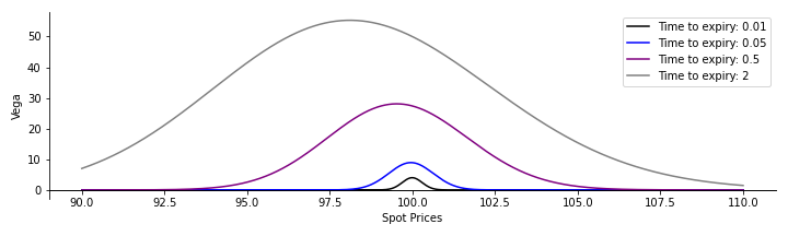
Vega quantifies the sensitivity of an option price to volatility, $\sigma$. $$ \nu = \frac{\partial C}{\partial \sigma} $$ Vegas for call and put options are strictly positive, since volatility always positively affects the option price. Options typically have the largest vega when options are far from expiry, as the variance of the probability distribution of the asset at expiry scales as $\sigma \tau$. Furthermore, vega tends to be largest when the spot price is close to the strike price.
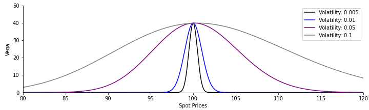
Vega of an option
While the functional form of vega for call options is $$ \nu_{\text{call}} = S n(d_1) \frac{\partial d_1}{\partial \sigma} - K e^{-r\tau} n(d_2) \frac{\partial d_2}{\partial \sigma}, $$ and for put options it is $$ \nu_{\text{put}} = -S n(d_1) \frac{\partial d_1}{\partial \sigma} + K e^{-r\tau} n(d_2) \frac{\partial d_2}{\partial \sigma}, $$ it is much more common to use the approximation $$ \tilde{\nu} = S n(d_1) \sqrt{\tau} $$ for both call and put options. This is because vega only concerns the sensitivity to volatility, and not price or time decay. As a result, the term in the Black-Scholes price of the form $SN(d_1)$ is the most sensitive quantity to changes in volatility, and the use of $\sqrt{\tau}$ comes from more practical considerations of what determines the volatility sensitivity inside $\frac{\partial d_1}{\partial \sigma}$.
Theta ($\Theta$)
Theta, otherwise referred to as `time-decay', is the sensitivity of the price of an option with respect to the time to expiry. $$ \Theta = -\frac{\partial C}{\partial \tau} $$ The minus sign comes from the fact that the time to expiry, $\tau$, is strictly decreasing. Since $\tau = T-t$, $\Theta$ is equivalent to the change of the option price with respect to time.
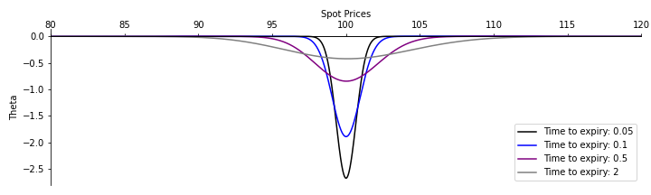
Theta of an option
The option price decays more rapidly the closer the option is to expiry, and if the spot price is close to the strike price. If the risk-free rate is zero, $\Theta$ is the same for calls and puts. The functional form of $\Theta$ for call options is $$ \Theta_{\text{call}} = -\frac{S \sigma n(d_1)}{2 \sqrt{\tau}} - rK e^{-r\tau} N(d_2) $$ and for put options it is $$ \Theta_{\text{put}} = -\frac{S \sigma n(d_1)}{2 \sqrt{\tau}} + rK e^{-r\tau} N(-d_2). $$ It is possible for put options to have a positive $\Theta$, provided there is a risk-free rate that is greater than zero. To understand why, suppose we are holding a put option and suppose that the spot price remains constant until expiry. Since the market expects the underlying to increase by the risk-free rate, as the option approaches expiry the expected increase of the underlying price by risk-free rate decreases, which increases the value of the put in time. Under most conditions, $\Theta$ is negative when we are long an option, and positive when we are short an option. In fact, for American options this always holds, since the option can be exercised at any time and the interest rate argument above does not apply.
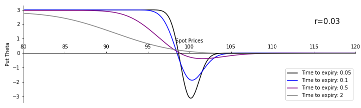
Theta of a put option with positive interest rates
The value of an option consists of two components, usually called the intrinsic component and the extrinsic component. The intrinsic value of an option is the payoff if the option was executed immediately. The extrinsic component is the premium the market is willing to pay above the intrinsic value, based upon the probability that the option will increase in value before expiry. $\Theta$ quantifies the change in the extrinsic value over time. Given that the extrinsic value of an option typically decreases over time, the extrinsic value is often called the time value of the option.