Mathematics
Random Variables I
This course is designed for those who are interested in understanding and applying discrete random variables in the context of quantitative finance. The second part of the series, Random Variables II, will cover continuous random variables and will build upon the intuition developed in this course. The concept of random variables underpin much of modern finance, and as such a deep working knowledge of random variables is of paramount importance.
The random variable is a concept that lies at the heart of quantitative finance. A random variable is a quantity that can take on different values with certain probabilities. For example, a die roll is a random variable with outcomes $\{1,2,3,4,5,6\}$. For a fair die, all outcomes are equally likely with probability $\frac{1}{6}$. The mathematical framework of random variables gives us the toolset to analyse uncertain events, make predictions and assess the likelihood of certain events occurring. Let's dive into some mathematics. Let us define a random variable, $X$. Measuring $X$ gives us an outcome $X_k$ with probability $p_k$. An equivalent way of denoting $p_k$ is to write $P(X = X_k)$, the probability that $X$ takes on the specific value $X_k$. $P$ is known as the probability mass function, which is a function of the space that the outcomes lie on - in the case of a die roll, it is the natural numbers. You can draw a probability mass function by plotting the probabilities on the y-axis, and outcomes on the x-axis. An example of the probability mass function is displayed below.
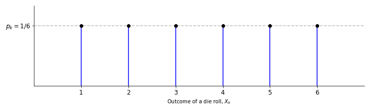
The probability mass function for a single die roll.
The expected value of a random variable is defined as $$ \text{E}[X] = \sum_{k=1}^{N} p_k \cdot X_k. $$ $\text{E}[X]$ can be read as "expectation of $X$". The expected value is equivalent to the mean of the random variable. "Expected value of $X$", "mean of $X$", and "expectation of $X$" are used interchangeably.
An important property of expected value is linearity. Linearity of expectation means that $$\text{E}[X+Y] = \text{E}[X] + \text{E}[Y]$$ for two random variables X and Y. This property will often simplify calculations significantly, so it is definitely worth remembering.
The variance of a random variable is a quantitative measure of how much a random variable tends to deviate from its expected value. Random variables with higher variance are more spread out from their expected value. The formal definition is $$ \text{Var}(X) = \sum_{k=1}^{N} p_k \cdot (X_k - \text{E}[X])^2. $$ We can see that the definition of variance is actually an expectation: the expectation of $(X - E[X])^2$. As a result, it is often written as $$ \text{Var}(X) = \text{E} \hspace{-1mm} \left[ (X - \text{E}[X])^2 \right]. $$
The standard deviation, $\sigma$, is defined as the square root of the variance. $$\text{Var}(X) = \sigma^2$$ Why would we need to define such a quantity? Well, standard deviation has an attractive property: it is expressed in the same units as the mean. As a result, it's the most commonly used measure of the deviation of a random variable. The final two properties we will cover in this section are covariance and correlation. The covariance measures the joint variability of several random variables. The covariance between two random variables $X$ and $Y$ is defined as $$ \text{Cov}(X,Y) = \text{E}\left[ \left( X - \text{E}[X] \right) \left( Y - \text{E}[Y] \right) \right] $$ The correlation coefficient, $\rho$ of two random variables $X$ and $Y$ is the covariance normalised by the product of the standard deviations $X$ and $Y$, $\sigma_X$ and $\sigma_Y$ respectively. $$ \rho_{XY} = \frac{\text{Cov}(X,Y)}{\sigma_X \sigma_Y}. $$ To finish, let's look at an example. The table below contains five joint measurements of $X$ and $Y$.
| $X$ | $Y$ |
|---|---|
| 2 | 3 |
| 2 | 2 |
| 3 | 4 |
| 3 | 5 |
| 5 | 6 |
Example: the Poisson distribution
The Poisson distribution describes the probability of a number of events occurring in a given time interval, if the events are independently occurring with a mean rate $\lambda$. The Poisson distribution is often used in finance to model events, such as incoming updates from an exchange. The probability of $k$ events occurring in a time interval is given by $$ f(k; \lambda) = P(X=k) = \frac{\lambda^k e^{-\lambda}}{k!}. $$ Since there cannot be a fractional number of events occurring in an interval, the Poisson distribution is a discrete distribution. The probability mass function of the Poisson distribution is shown in the image below.
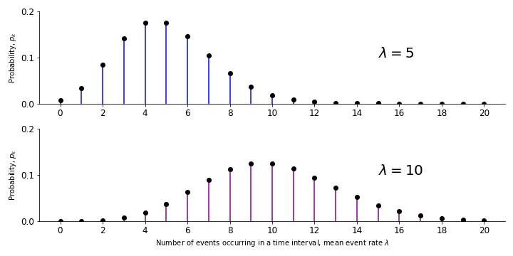
The probability mass function of the Poisson distribution
The expected value of the Poisson distribution is $$ E[X] = \lambda $$ and the variance is $$ \text{Var}(X) = \lambda. $$ Once again, it is worth proving these relationships for yourself. You will need the definitions of expected value and variance for discrete random variables in the previous section.