Mathematics
Random Variables II
Developing the intuition developed in Random Variables I, we extend this concept to continuous random variables. Continuous random variables underpin much of quantitative finance, and are used in fields such as asset modelling and options pricing. This section will serve as a foundation which we will build upon extensively in later sections.
Unlike discrete random variables, continuous random variables have an uncountably infinite number of potential outcomes. For example, the temperature in Paris tomorrow is a continuous random variable since it can take the value of any real number greater than absolute zero. Whereas in the case of discrete random variables we consider a countable set of outcomes $\{X_k\}$ with probabilities $\{p_k\}$, for continuous variables we need to consider the probability distribution function, $f(x)$. Instead of considering the probabilities of specific outcomes, we consider the probabilities of ranges of outcomes. In this section we will be exploring the properties of the continuous random variables $X$, $Y$. The probability of the random variable $X$ lying between the bounds $a$ and $b$ is given by $$ P(a < X \leq b) = \int_{a}^{b} f_X(x) dx. $$ The cumulative distribution function, $F(k)$ gives the probability of the random variable $X$ lying below an upper bound $k$. $$ F_X(k) = P(X \leq k) = \int_{-\infty}^{k} f_X(x) dx $$ A useful property of the cumulative distribution is $$ P(a < X \leq b) = F_X(b) - F_X(a). $$ As an exercise it is worth proving this equation for yourself. The expected value of $X$ is defined as $$ E[X] = \int_{-\infty}^{+\infty} x f(x) dx. $$ Letting $E[X] = \mu_X$ for more neat notation, the variance of $X$ is equal to $$ \text{Var}(X) = E[(X- \mu_X)^2] = \int_{-\infty}^{+\infty} (x-\mu_X)^2 f(x) dx $$ and the standard deviation is equal to the square root of the variance, same as in the case of discrete random variables. $$ \sigma = \sqrt{\text{Var}(X)} $$
Example: Uniform Distribution
The uniform distribution, $f_{[a,b]}(x)$ is a probability distribution where all outcomes in the sample space occur with equal probability. It is defined as $$ f_{[a,b]}(x)=\begin{cases} \frac{1}{b-a}, & \text{if $a \leq x \leq b$}.\\ 0, & \text{otherwise}. \end{cases} $$ The probability distribution function, $f_X(x)$ and cumulative distribution function, $F_X(x)$ are displayed below.
![The probability distribution function, $f_{[a,b]}(x)$, (top) and cumulative distribution function, $F_{[a,b]}(x)$, (bottom) of the uniform distribution with $a=-1$, $b=1$.](/media/course_images/uniform.png)
Distribution functions for the uniform distribution
Example: Normal Distribution
Here we introduce one of the most important distributions in quantitative finance. By the time you come to interviewing, you should know the normal distribution inside and out. The normal distribution is widely used across many disciplines, including finance. For example, a popular way to model returns on assets is by assuming that the log of the returns are normally distributed. A significant reason why the normal distribution is so popular is the Central Limit Theorem, which we will cover next. The normal probability density function is $$ f(x) = \frac{1}{\sigma \sqrt{2 \pi}} \exp \left(-\frac{1}{2} \left(\frac{x-\mu}{\sigma}\right)^2 \right). $$
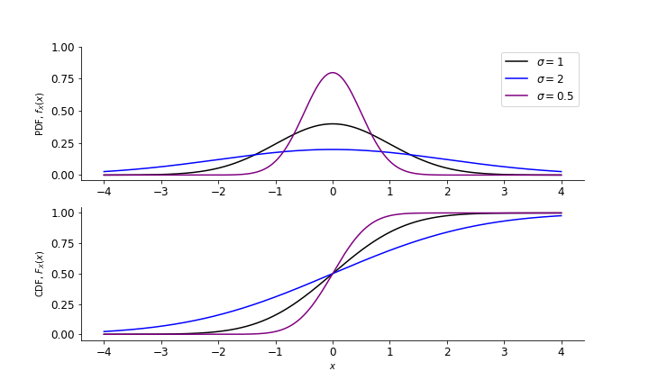
Distribution functions for the normal distribution
The expected value of the normal distribution is $$ E[X] = \mu $$ and the variance is $$ \text{Var}(X) = \sigma^2. $$ Using the integral definitions of expected value and variance, prove the two above equations for yourself.
You will often see the normal distribution with mean $\mu$ and variance $\sigma^2$ denoted as $N(\mu, \sigma)$, and we will use this notation frequently through the rest of the courses. A useful rule-of-thumb for the normal distribution is the empirical rule, also called the $63.7-95-99.7$ rule: which is a rule used to remember the percentage of values that lie within an interval estimate in a normal distribution. In particular, the intervals here are $\sigma$, $2\sigma$ and $3\sigma$ away from the mean.
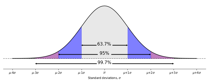
The empirical rule for the normal distribution