Stochastic Calculus

In this section, we go further on random processes and outline the basics of stochastic calculus. We leave a fully rigorous treatment of this section to mathematicians, and instead focus on the key ideas. First, let's think about what Brownian motion actually is. Consider a collection of random variables $\{ X_t \}$ for $0 \leq t \leq T$. $X_0$ is a well-defined value - the initial value of the Brownian motion. $X_t$ is a normally distributed random variable with mean $X_0$ and variance $\sigma^2 t$ $$ X_t \sim N(0, \:\sigma^2 t). $$ We also have that for some other time $s \lt t$, $X_t - X_s$ is a normally distributed random variable with variance $\sigma^2 (t-s)$. $$ X_t - X_s \sim N(0, \:\sigma^2 (t-s)) \: \forall s \lt t. $$ Furthermore, the random variables $$ X_t - X_s, \: X_s $$ are completely independent of each other. In fact, $X_t - X_s$ is independent of $X_s$ and all $X_r$ with $r \lt s$. This is known as the Markov property. The sequence of random variables with the property that $$ X_t - X_s \sim N(0, \sigma^2 (t-s)) $$ is a Brownian motion. Let us define a standard Brownian motion as a sequence of random variables $\{ W_{t>0}\}$ such that $W_0=0$ and $$ W_t - W_s \: \forall s \lt t $$ is a normally distributed random variable that is independent of all $ W_{r\leq s} $.

Quadratic Variation

The quadratic variation of a function is the sum of the squares of its moves at each time step. For regular continuous and differentiable functions, the quadratic variation is always zero. Suppose we take an interval $[0, T]$ and partition the interval into $n$ equally-sized partitions. The length of a partition is $$ l = t_{i+1} - t_i = \frac{T}{n}. $$ The quadratic variation is defined as $$ X_n = \sum_{i=0}^{n-1} (f(t_{i+1}) - f(t_i))^2 \geq 0 $$ Now, let's insert Brownian motion into the above function $$ X_n = \sum_{i=0}^{n-1} (W_{t_{i+1}} - W_{t_i})^2 $$ $$ \text{E}[X_n] = \text{E} \left[ \sum_{i=0}^{n-1} (W_{t_{i+1}} - W_{t_i})^2 \right] $$ $$ \text{E}[X_n] = \sum_{i=0}^{n-1} \text{E} \left[ (W_{t_{i+1}} - W_{t_i})^2 \right]. $$ Now, we know that $$ W_{t_{i+1}} - W_{t_{i}} \sim N(0, \frac{T}{n}) $$ and $$ \text{E} \left[ X^2 \right] = \text{Var}(X) + \text{E}[X]^2. $$ So, we know that $$ \text{E} \left[ (W_{t_{i+1}} - W_{t_i})^2 \right] = \text{Var}\left( W_{t_{i+1}} - W_{t_i} \right) + \text{E}\left[ W_{t_{i+1}} - W_{t_i} \right] = \frac{T}{n}. $$ Therefore, $$ \text{E}\left[ X_n \right] = \sum_{i=0}^{n-1} \text{E} \left[ (W_{t_{i+1}} - W_{t_i})^2 \right] = T. $$ We do not show it here, but it is possible to show that the variance of the quadratic variation goes to zero as $n$ goes to infinity. Therefore the quadratic variation of the Brownian motion converges to a finite value $T$.

Ito's Lemma

Ito's Lemma is a fundamental concept in stochastic calculus, which is widely used in quantitative finance, particularly in the modelling of financial markets and the pricing of derivatives. This lemma provides a way to differentiate and integrate functions of stochastic processes. Let's $W_t$ be a Brownian motion. The set of random variables $\{ X_t \}$ satisfies the stochastic differential equation $$ \text{d}X_t = \mu (t, X_t) \: \text{d}t + \sigma (t, X_t) \: \text{d}W_t $$ provided that $$ X_{t+h} - X_t - h\mu(t, X_t) - \sigma (t, X_t)(W_{t+h} - W_t) $$ is a random variable with mean and variance on the order of $h$. What does `order of $h$' mean exactly? A function or variable is on the order of $h$ (usually written $o(h)$) if it converges to zero faster than $h$. Let's compare the stochastic differential equation with the standard differential equation we are familiar with. The definition of a standard derivative is $$ \lim_{h \rightarrow 0} \frac{f(x+h) - f(x)}{h} = \frac{\text{d}f(x)}{\text{d}x} $$ or equivalently, $$ f(x+h) - f(x) - h \frac{\text{d}f(x)}{\text{d}x} = o(h). $$ Notice how similar it is to $$ X_{t+h} - X_t - h\mu(t, X_t) - \sigma (t, X_t)(W_{t+h} - W_t) = o(h). $$ In fact, setting $\sigma=0$ recovers the regular definition of the derivative $$ \frac{\text{d}X_t}{\text{d}t} = \mu (t, X_t). $$ Ito's Lemma is to stochastic calculus what the chain rule is to classical calculus. We will make us of Taylor's theorem - that is, for $x$ close to $a$, $$ f(x) = f(a) + (x-a)f'(a) + \frac{1}{2} (x-a)^2 f''(a) + o(|x-a|^3). $$ Where the classical derivative requires a linear Taylor expansion, we require a quadratic expansion here. This requirement is closely related to the fact that the quadratic variation is nonzero, which we discovered earlier. Now, let us substitute $X_{t+h}$ for $x$ and $X_t$ for $a$, $$ f(X_{t+h}) - f(X_t) = f'(X_t)(X_{t+h} - X_t) + \frac{1}{2} f''(X_t)(X_{t+h} - X_t)^2 + \varepsilon $$ Recall that $$ \text{d}X_t = \mu(t, X_t) \text{d}t + \sigma (t, X_t) \text{d}W_t. $$ This implies $$ X_{t+h} - X_t = h\mu(t, X_t) + \sigma \sqrt{h} N(0,1) + \varepsilon. $$ It is worth remembering that $$ \text{d}W_t = W_{t+h} - W_t \sim \sqrt{h} N(0,1). $$ Now, let us substitute back in to the Taylor expansion $$ f(X_{t+h}) - f(X_t) = f'(X_t) \left[ \mu h + \sigma \sqrt{h} N(0,1) \right] + \frac{1}{2} f''(X_t) \left[ \left(\mu h + \sigma \sqrt{h} N(0,1) \right)^2 \right]. $$ The only term that survives the square expansion is $h \sigma^2$. So, $$ f(X_{t+h}) - f(X_t) = f'(X_t) \left[ \mu h + \sigma \sqrt{h} N(0,1) \right] + \frac{h \sigma^2}{2} f''(X_t) $$ $$ \text{d}f(X_t) = f'(X_t) \left[ \mu \: \text{d}t + \sigma \: \text{d}W_t \right] + \frac{\sigma^2}{2} f''(X_t) \: \text{d}t $$ $$ \text{d}f(X_t) = \left[ \mu f'(X_t) + \frac{\sigma^2}{2} f''(X_t) \right] \text{d}t + \sigma f'(X_t) \: \text{d}W_t $$ and that's it! We have generalised the chain rule for stochastic processes. Now, let's write the formal definition of Ito's Lemma. Let $X_t$ be an Ito process satisfying $$ \text{d}X_t = \mu(X_t, t) \text{d}t + \sigma(X_t, t) \text{d}W_t $$ and let $f(x,t)$ be a twice differentiable function. Then, $f(X_t, t)$ is an Ito process and $$ \text{d}f(X_t, t) = \frac{\partial f}{\partial t}(X_t, t) \text{d}t + \frac{\partial f}{\partial X_t} (X_t, t) \text{d}X_t + \frac{1}{2} \frac{\partial^2 f}{\partial X_t^2} (X_t, t) \text{d}X_t^2. $$ where $$ dt^2 = 0 $$ $$ dW dt = 0 $$ $$ dW^2 = dt. $$

Example: Geometric Brownian Motion

Geometric Brownian motion is a continuous-time stochastic process that is commonly used in quantitative finance, particularly in the modelling of asset prices. It's a type of stochastic process that exhibits both the properties of Brownian motion and the proportional scaling typical of geometric sequences. Whereas increments in standard Brownian motion are additive, incremental changes in geometric Brownian motion are proportional to its current value. Geometric Brownian motion has several useful properties for modelling assets. It cannot take negative values, and the incremental movements are percentage movements rather than absolute movements. The stochastic differential equation for geometric Brownian motion is $$ \text{d}X_t = \mu (t, X_t) X_t \: \text{d}t + \sigma (t, X_t) X_t \: \text{d}W_t $$

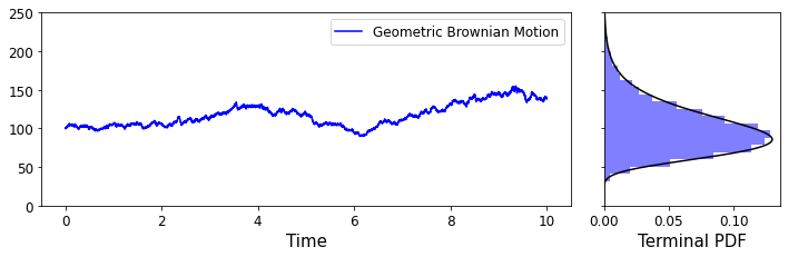
Diagram illustrating Geometric Brownian Motion

×

❮

❯

The terminal probability density function of the geometric brownian motion is the lognormal distribution, defined as $$ f(x) = \frac{1}{sx\sqrt{2\pi}} \exp \left( - \frac{\log^2(x)}{2s^2} \right) $$ The expected value of the lognormal distribution is $$ \text{E}[X] = \exp \left( \mu T + \frac{\sigma^2}{2} T\right) $$ and the variance is $$ \text{Var}(X) = \left[ \exp(\sigma^2 T) - 1 \right] \exp \left( 2 \mu T + \sigma^2 T \right). $$