Mathematics
Moments
Moments generalise the properties of the probability distribution function, and are quantitative measures associated with the shape of a function. In this section we will cover the first four moments: expected value, variance, skewness and kurtosis, ending with a discussion of a key concept in quantitative finance: the concept of fat tails. Moments are an extremely useful tool to characterise the risk and returns of assets, and frequently come up in many other areas in quantitative finance.
Moments generalise the properties of the probability distribution function, and are quantitative measures associated with the shape of a function. The $n$th moment about some constant, $c$, is defined by $$ \mu_n(c) = E[(X-c)^n] = \int_{-\infty}^{+\infty} (x - c)^n f(x) \hspace{1mm} \text{d}x $$ When $c=0$, moments are known as {\it raw} moments. The only raw moment that is used in practice is the expected value. The second order moment is typically taken about the expected value, $c = \mu_X$ of the probability distribution function. In general, we define the {\it centralised} moment to be the moment where $c = \mu_X$. The centralised second order moment is equal to the variance. $$ Var(X) = \mu_2(\mu_X) = \int_{-\infty}^{+\infty} (x - \mu_X)^2 f(x) \text{d}x $$ The third and forth moments are frequently used in finance, are centralised and standardized according to the variance. The $n$th standardized moment is defined as $$ \frac{\mu_n}{\sigma^n} = \frac{E[(X - \mu)^n]}{\sigma^n} $$ The third-order moment is known as the skewness, which is a measure of the asymmetry of the distribution about its mean. A distribution that is skewed to the left will have a negative skewness, and one that is skewed to the right will have positive skewness. A distribution that is symmetric about its mean will have a skewness of zero.
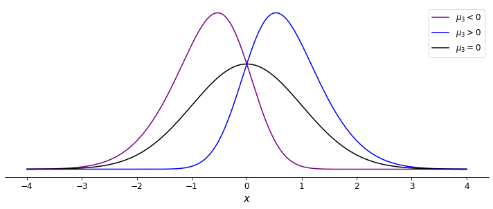
Demonstration of skewness
The fourth-order moment is known as the kurtosis, which describes the "tailedness" of a distribution - that is, the propensity of a distribution to produce outliers. Commonly, the `excess kurtosis' is defined as the kurtosis relative to a normal distribution. The normal distribution has a kurtosis of 3, so the excess kurtosis is simply the kurtosis minus 3. A lower kurtosis indicates a higher propensity for the distribution to produce outliers.
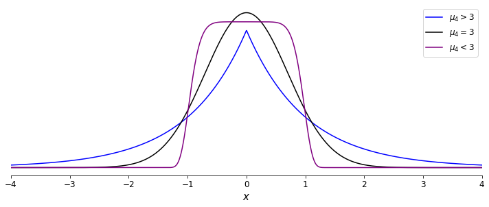
Demonstration of kurtosis
Example: Verifying the Central-Limit Theorem
The central limit theorem demonstrates that if we have some complex phenomena determined by the sum of an effectively infinite number of random factors, we can model the phenomena as being a normally distributed random variable. In particular, we can model the returns of financial assets as being normally distributed. Let's look at historical data of the returns of the S&P 500 and see if this model holds up with reality.
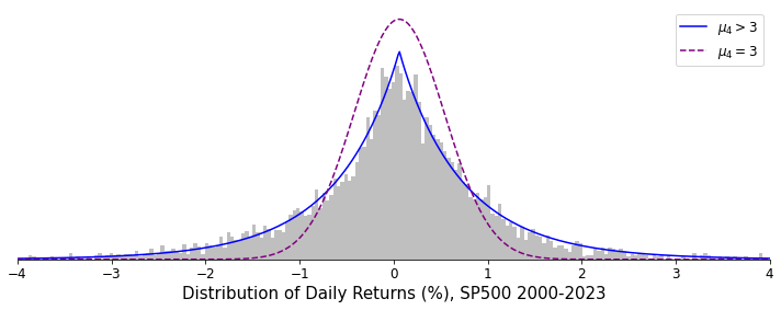
A histogram of S&P 500 returns compared to the normal distribution
So, what went wrong? The central limit theorem assumes that the underlying random variables are independent and identically distributed. Clearly, this assumption cannot be true. In the case of financial returns, successive returns are often not independent. Financial markets have memory, and past returns can influence future returns, especially over short and medium-term horizons. Market returns can also be influenced by various factors that change over time, like economic policies, market sentiment, and global events, leading to non-identical distribution of returns.
Fatter tails indicate a higher likelihood of outlier values compared to what the normal distribution would predict. This characteristic is common in financial returns and signifies a higher frequency of extreme market movements compared to what we would expect if financial returns were normally distributed. Examples of these extreme market movements are Black Monday (1987), the 2008 Financial Crisis and the 2020 Stock Market Crash.