Mathematics
Random Processes
Random processes lie at the core of quantitative finance, with the price of an asset in time being the prototypical example of a continuous-time random process. Portfolio management, while being a vast industry worth billions of dollars, boils down to studying the properties of linear combinations of real-world random processes. To put it short, a strong grasp of random processes is absolutely essential.
Random processes are a collection of random variables indexed in time. A Markov chain is actually an example of a random process. In particular, it is a discrete-time random process. To see this, suppose a Markov chain has initial state $X_0$. After the first transition, we label the new state $X_1$ and label every subsequent state $X_i$ with increasing values of $i$. Then, by definition the set $\{ X_i, i=0,1,2,3... \}$ is a random process with discrete time steps. It is most rigorous to think of Markov chains as a random time-dependent process, and the expected hitting time calculations we covered in the previous section are calculations concerning the behaviour of a time-dependent process. Let us consider a new discrete-time random process - the random walk. Suppose that we discretize time by some tiny interval of length $\Delta$. For every interval, we generate an independent random variable where $$ X_{k} = \begin{cases} \sqrt{\Delta} \hspace{4mm} \text{with probability 0.5}\\ - \sqrt{\Delta} \hspace{2mm} \text{with probability 0.5}. \end{cases} $$
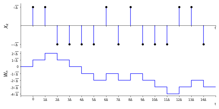
Diagrams illustrating the random walk.
Now, consider that at every time interval, we move up or down according to the realised value of $X_k$. We will either take a step forward or a step backward with equal probability and with size $\sqrt{\Delta}$. This random process is known as the {\bf random walk}, denoted $W_n$. It is the cumulative sum of $X_k$ up to time $n$. $$ W_n = \sum_{k=0}^{n} X_k $$
Since $\Delta$ is the size of our time intervals, $n\Delta$ is infact just the time at the $n$th interval, $n\Delta = t$. As we shrink the interval time into the limit $\Delta \rightarrow 0$, we see that $n \rightarrow \infty$. Now, recall the central limit theorem $$ \lim_{n \rightarrow \infty} \frac{S_n - n \mu}{\sigma \sqrt{n}} \sim N(0, 1) $$ Given that $\{ X_k \}$ are independent and identically distributed, this theorem applies. Here, $\sigma$ is the standard deviation of $X_k$, which is $\sqrt{\Delta}$. So, we have $$ \lim_{n \rightarrow \infty} \frac{W_n}{\sqrt{n\Delta}} \sim N(0, 1) $$ or, equivalently $$ \lim_{n \rightarrow \infty} \frac{W_t}{\sqrt{t}} \sim N(0, 1). $$
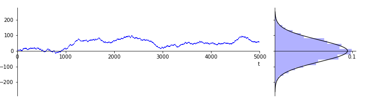
Probability distribution produced by the random walk
What the above equation tells us is that in the limit of $\Delta \rightarrow 0$, the random walk obeys a normal distribution in which the standard deviation grows in time as $\sqrt{t}$. This process is known as Brownian motion, and is used extensively in the modelling of assets and the pricing of derivatives. We will go deeper on this topic in the next section on stochastic calculus.