Interest Rates

So far, we have left out an important property in markets which will affect our models. We have assumed that currencies have a constant value over time. However, in reality, currencies are subject to interest rates which decrease or increase their value. We will incorporate interest rates by using a theoretical financial instrument called the risk-free bond. The risk-free bond behaves in a simple way - it's value changes in time according to the following equation $$ B_t = B_0 e^{r t}. $$ Here, $r$ is known as the risk-free rate, which can be thought of the rate of return that you can expect without bearing any risk. Riskless assets do not exist in reality of course, but the closest example might be a U.S. Treasury Bond. These bonds are often treated as riskless as they are backed by the American government, and if the American government defaults on it's treasury bonds there are bigger issues to worry about than pricing options. Owning assets such as stocks involve more risk - the risk of the company going bankrupt for example - and therefore we should generally expect a rate of return greater than $r$ for holding such risky assets. What the risk-free bond represents is the rate at which the value of a currency changes. Suppose we have an extremely stable asset which has volatility equal to zero. According to what we have done previously, the stock price should be constant. However, since the value of the currency is changing according to the risk-free rate, then $$ S_t = S_0 e^{rt}. $$ If we consider a stock with some volatility $\sigma > 0$, the expected future stock price is $$ \text{E}[S_t] = S_0 e^{rt}. $$

Put-Call Parity

A common contract in finance is the forward, which is an agreement to buy or sell an asset at some future date at some specified strike price, $K$. This contract is a binding agreement that obligates the parties to fulfil the transaction as agreed, regardless of the prevailing market price of the underlying asset at the time of settlement. The value of a forward contract is determined by the expected future value of the stock when the contract expires $F = \text{E}[S_t]$, which we know now is equal to $S_0 e^{rt}$. An important concept involving options and forward contracts is {\it put-call parity}, which is a relationship between a portfolio consisting of one call option and short one put option and a forward contract. Put-call parity states that $$ C - P = e^{-rt} (F - K) $$ and since the discounted forward price is equal to the current spot price, $e^{-rt}F = S_0$, we have $$ C - P = S_0 - Ke^{-rt}. $$ To understand why this relationship between a forward contract and options exists, consider the following. If at expiry the spot price is above the strike price, then you purchase the asset for the strike price. However, if at expiry the spot price is below the strike price, then the owner of the put contract you sold will exercise and you are obligated to purchase the asset for the strike price. Therefore, regardless of the outcome you will be purchasing the asset for the strike price - which is a forward contract and has value $(F-K)$. What remains is to discount the interest rate to obtain the value before expiry. We will use this relationship later on after deriving the Black-Scholes price for a call option to derive the price of a put option.

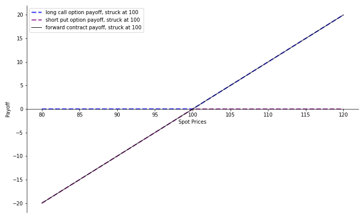
Demonstration of Put-Call Parity

×

❮

❯

Binomial Trees

For binomial trees, a risk-free rate adjusts the probabilities of a stock going up or down in a time step. Let us define $S_0$ as the stock price at $t=0$, and $S_+$ and $S_-$ as the stock price at the next time step $t=\tau$ corresponding to whether the stock goes up or down respectively. Whereas before we found that $p=0.5$, now we have $$ E[S_\tau] = S_0 e^{r\tau} = p S_+ + (1-p)S_-. $$ We require that at every step in the binomial tree has a step size such that $$ S_- < S_0 e^{r\tau} < S_+ $$ otherwise the stock will go either up or down in value with probability 1. If that happens, we can obtain a risk-free profit by buying or selling the asset now, and then closing our position on the next time step to gain the difference. Since risk-free profits don't exist in reality, we must enforce the constraint above. The probabilities are therefore determined from the risk-free rate, the size of the time step and the size of the discontinuous jumps between stock prices at each time step. To price an option for a binomial tree with a single time step and two possible outcomes we can use these new probabilities to calculate the expected future payoff. Keep in mind that since we're pricing an option at $t=0$, so we need to discount the interest rate by the discount factor $e^{-r\tau}$ to get today's value. $$ C_0 = e^{-r\tau} \left[ \: p g(S_+) + (1-p) g(S_-) \: \right] $$ Interest rates are incorporated into the binomial tree model by simply adjusting $p$ and then using the binomial distribution to determine future probabilities as before.

The Lognormal Model

Given a risk-free rate $r$ we have $$ \text{E}[S_t] = S_0 e^{rt}. $$ We can include an additional term in our equation for the normal model $$ \log S_T = \log S_0 + (\mu - \frac{1}{2} \sigma^2) T + \sigma \sqrt{T} \: N(0, 1). $$ The parameter $\mu$ is known as the drift, and describes the average rate of change of the asset price over time. As we mentioned earlier, we would expect $\mu$ to be greater than $r$ as the asset is risky and we expect some compensation for bearing that risk. Now, we want to find the drift $\mu$ which makes the expected value of the probability distribution at expiry equal to $S_0 e^{rT}$. $$ S_T = S_0 e^{\left( \mu - \frac{1}{2} \sigma^2\right)T + \sigma \sqrt{T} N(0,1)} $$ $$ \text{E}[S_T] = S_0 e^{rT} = \text{E}\left[S_0 e^{\left( \mu - \frac{1}{2} \sigma^2\right) T + \sigma \sqrt{T} N(0,1)}\right] $$ $$ \text{E}\left[S_0 e^{\left( \mu - \frac{1}{2} \sigma^2\right) T + \sigma \sqrt{T} N(0,1)}\right] = S_0 e^{\left( \mu - \frac{1}{2} \sigma^2\right) T} \cdot \text{E} \left[ e^{\sigma \sqrt{T} N(0,1)} \right] $$ So, we have $$ S_0 e^{r T} = S_0 e^{\mu T} $$ which implies $$ \mu = r. $$ Now we have a lognormal model which incorporates interest rates. This model is frequently used in quantitative finance and underpins the Black-Scholes model for pricing options. $$ \log S_T = \log S_0 + (r - \frac{1}{2} \sigma^2) T + \sigma \sqrt{T} \: N(0, 1). $$ See that we price options according to risk-neutral pricing, which assumes that all assets grow at the risk-free rate. The reason we do this is if we assume that the expected value of $S_t$ is anything other than $S_0 e^{rt}$, there are arbitrage opportunities. We could obtain a risk-free profit by buying the asset with the larger drift and shorting the asset with the smaller drift. We will see idea again when we derive the Black-Scholes equation in the next section.