Options Pricing
Binomial Pricing Model
In this section we will look at our first model for pricing options. This model involves constructing a tree of prices into the future, and assigning probabilities to the asset going up or down in each time step. At expiry, we will then have a set of prices and probabilities, enabling us to calculate the option price. This model underpins the more advanced models that we will see in later sections. Nonetheless, this model is still frequently used to calculate option prices in large financial institutions.
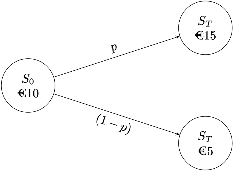
Consider an asset $S$. Suppose that at time $t=0$ the value of the stock is €10. At $t=T$ the value of the stock will either be €15 or €5, with probability $p$ and $1-p$ respectively. We want to price an option $C$ which is struck at $K=€10$.
One-step binomial model
We can construct a portfolio, consisting of an option and the underlying stock, which has the same value at $t=T$ regardless of whether the stock is €5 or €15. Let us define the portfolio $P$ $$ P = \Delta S - C $$ which is long $\Delta$ of the underlying stock and short one call option. If $S_T = €15$, then the option payoff is €5 and the value of the portfolio is $$ P = 15\Delta - 5 $$ and if $S_T = €5$, then the option is not exercised and $$ P = 5\Delta. $$ Since we require these portfolio values to be of equal value, we require that $\Delta = \frac{1}{2}$. So, we own half a stock in our portfolio and the portfolio value at $t=T$ is €2.5 regardless of the outcome. If the value of the portfolio at $t=T$ is equal to €2.5 in every possible outcome, then clearly it must also be worth €2.5 at $t=0$. We can now solve for the option price, $C$, at $t=0$. $$ 10 \Delta - C_0 = 2.5 $$ $$ C_0 = €2.5. $$ So, what did we just do here? We determined the price of an option by using a portfolio arbitrage argument. Suppose the option was actually priced at €3 at $t=0$. Holding the portfolio at $t=0$ gives us a risk-free profit at $t=T$. To see this, consider that the portfolio at $t=0$ is worth €2. But we know that the portfolio at $t=T$ must be worth €2.5. Holding the portfolio from $t=0$ to $t=T$ gives us a risk free profit of €0.5. Notice something very interesting - we can obtain values for the probabilities of the stock going up or down in value. The value of the option at $t=0$, $C_0$ is $$ C_0 = \text{E}[\text{Payoff}] = 5 \times p - 0 \times (1-p). $$ Given that we know now that $C_0 =$ €2.5, then $p=0.5$. This is known as risk-neutral pricing, and in fact setting $p=0.5$ will always agree with the portfolio method of pricing binomial trees. We will assume that the asset going up or down is equally likely, $p=0.5$, for the rest of the section. Now, we see that we can price options by modelling the stock as having discrete jumps into two potential outcomes. Clearly, in the real world stocks have many future values, not just two. So what can we do? We can add more steps to the tree.
Two-step binomial model
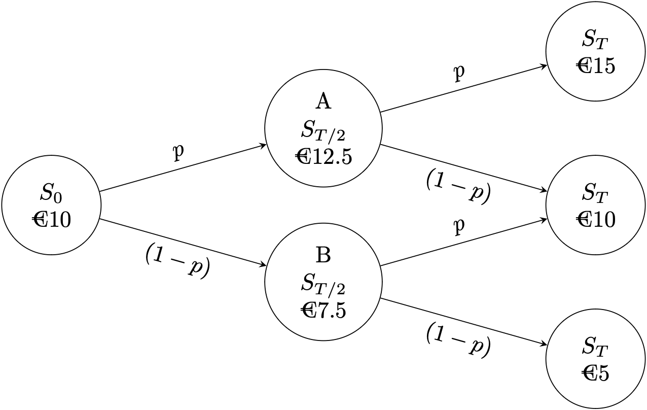
Here, we split the time step into two, with each time step having length $\frac{T}{2}$. Let's create a portfolio to price an option as before, struck at $K=€10$. Firstly, we see that the value of the option must be zero at the intermediate state B. This is because the only available outcomes are $S_T=€10$ and $S_T=€5$, both of which have zero payoff. For the intermediate state A, we can price the option by considering the portfolio $$ P = \Delta S - C $$ $$ P_{S_T = €15} = 15 \Delta - 5 $$ $$ P_{S_T = €10} = 10\Delta $$ $$ 15\Delta - 5 = 10\Delta \implies \Delta = 1. $$ Therefore, we solve for $C_{A}$ to get $$ C_{A} = 2.5. $$ Now we have the value of the portfolio value in the intermediate states of $A$ and $B$. We follow the same procedure again to get the portfolio value at $t=0$. $$ P_{A} = 12.5 \Delta - 2.5 $$ $$ P_{B} = 7.5\Delta $$ $$ 12.5\Delta - 2.5 = 7.5\Delta \implies \Delta = 0.5. $$ $P_A$ and $P_B$ are both worth €3.75. Once again, solve now for $C_0$ $$ P_0 = 0.5(10) - C_0 = 3.75 \implies C_0 = €1.25. $$ Again, we see that the option price is equivalent to setting the probability of an up-move equal to 0.5. We can derive the option price simply by considering that the probability of $S_T = €15$ is equal to $p^2 = 0.25$, with the payoff here equal to €5. All other outcomes result in zero payoff. Therefore, the option price is €1.25. Let's summarise everything we've learned before we move on. We derived an option price before expiry by constructing a model for the stock - one in which there are two outcomes at expiry - and created a portfolio of the option and $\Delta$ stocks which had the same value regardless of outcome at $t=T$. If the portfolio is worth $\$x$ in all possible outcomes at $t=T$, then it must also be worth $€x$ at $t=0$. Since we know the price of the stocks and the value of the portfolio, we simply solve $$ C_0 = \Delta S_0 - x $$ to get the option price. We see the value of the option implies that the probability of an up-move at each step in the tree is equal to 0.5. Setting $p=0.5$ is described as risk-neutral. The portfolio method of deriving the option price is tedious, and simply using the fact that $p=0.5$ simplifies our method of calculating the option price considerably. We can model the stock as a tree where at each step, the probability of the stock going up is $p=0.5$.
Four-step binomial model
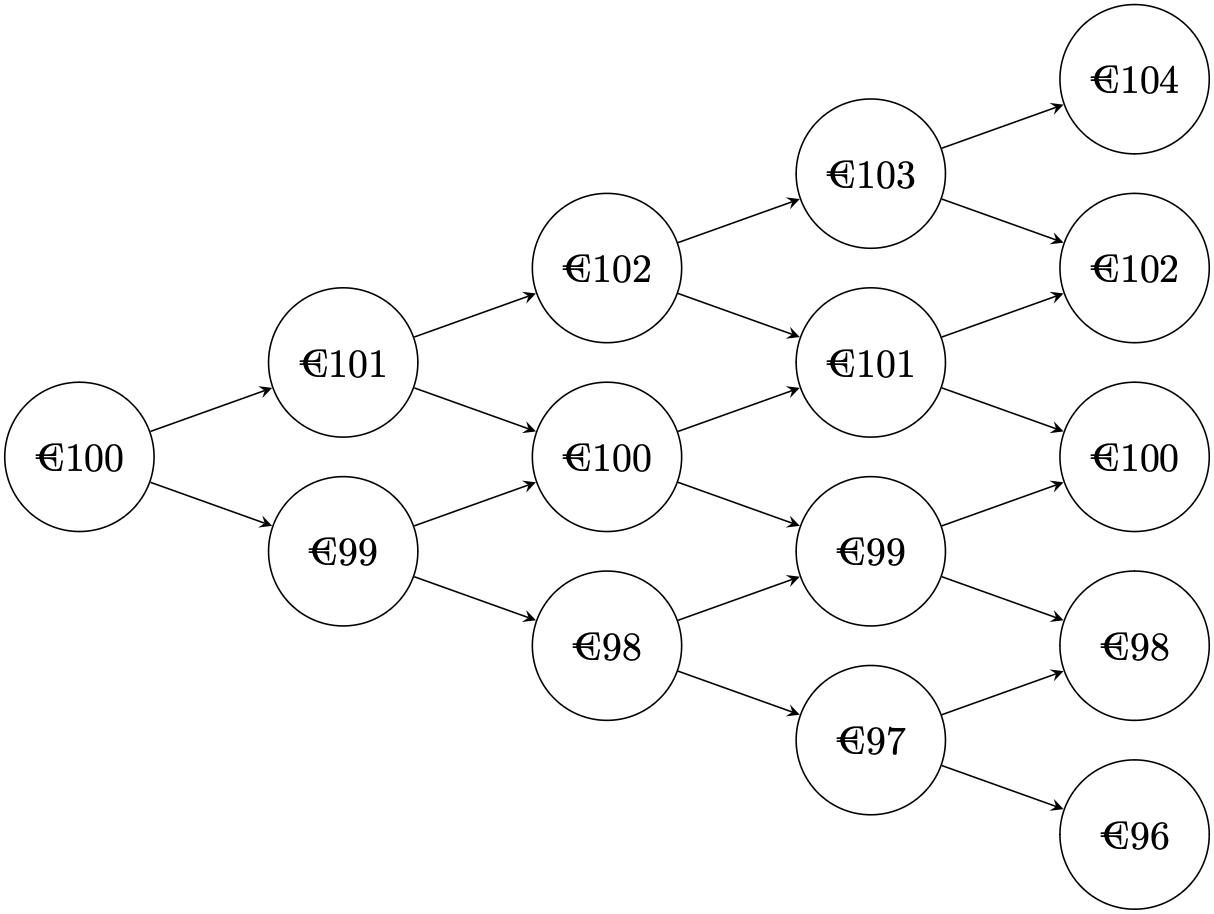
Now, we can assign a probability to each outcome - which was what we set out to do in the first place. The probability of the terminal stock price being €104 is equal to the probability of there being 4 up-moves without any down-moves. This is $$ P(S_T = €104) = \frac{1}{2^4} = \frac{1}{16}. $$ The probability of the stock price being €102 at $t=T$ is given by the probability of there being 1 down-move and 3 up-moves. We can calculate this by counting the number of combinations of 1 down-move and 3 up-moves there are in a set of 4 moves. Considering that each individual path from $t=0$ to $t=T$ occurs with probability $\frac{1}{2^4}$, $$ P(S_T = €102) = {4 \choose 1} \cdot \frac{1}{2^4} = \frac{1}{4}. $$
Now we will generalise this result for an arbitrary number of time steps. Let there be N steps in the binomial tree and at each step the price goes up or down by $q$. We want to write the stock value as a function of the number of up-moves $$ S(u) = S_0 + uq - (N-u)q = S_0 + (2u - N)q. $$ The probability of there being $u$ up-moves is $$ P(u) = {N \choose u} \frac{1}{2^N}. $$ Therefore, the expected payoff of an option is $$ \text{E}[\text{Payoff}] = \frac{1}{2^N} \sum_{u=0}^N {N \choose u} \text{Payoff}(S_0 + (2u - N)q). $$ The model we have described here is a very popular method of modelling the underlying asset in order to price derivatives. The probability distribution of $S_T$ can be calculated by using the binomial distribution for $n$ steps and $p=0.5$.