Trading
Statistical Arbitrage
Here we cover in-depth the concept of statistical arbitrage, with theory and a practical application. Statistical arbitrage has been an extremely popular and profitable trading strategy since it's discovery in the 1980s.
So far we have been discussing high-frequency trading: short-horizon trades that are dominated by quant firms. However, very often the same firms also trade over longer horizons, to diversify their strategy set and add further sources of income.
Statistical arbitrage differs from arbitrage in that it is not as likely to profit from every trade, however trading firms can construct trading strategies involving multiple correlated assets to profit more often than not. In this section we will outline the concept of statistical arbitrage, going through a real-world example and ending with a discussion detailing some practical considerations for implementing the strategy. Let's consider two assets: Coca-cola (KO) and Pepsi (PEP). The prices of these two assets are found to be correlated in time - when Pepsi increases in price it is more likely than not that Coca-cola will also increase in price. Securities with this property are described as cointegrated. Traders look for periods when the historical correlation deviates significantly from its typical behaviour. Deviations may be caused by market events, news, or other factors that temporarily impact the prices of the assets differently. When a deviation is identified, the trader takes a long position in the underperforming asset (expecting it to increase in value) and a short position in the outperforming asset (expecting it to decrease in value). The goal is to profit from the expected convergence of their prices. The strategy's success relies on the assumption that the historical correlation will eventually be restored. When the prices converge, the trader can close the positions, realizing a profit. However, it can also be the case that the market regime changes, and the prices will never converge. It is therefore not a guarantee that every trade will be profitable.
Let's now apply this strategy to a real-world example. We will download some daily stock data for Coca-cola and Pepsi. First, we will take a look at the time series of their stock prices between the period of November 2015 and November 2019.
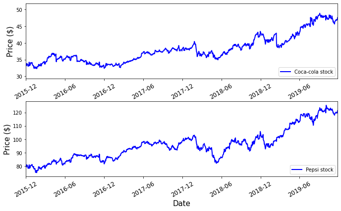
Time series of Pepsi and Coca-cola stock prices.
This looks promising! Generally, when Coca-cola goes up in price, so does Pepsi and vice versa. To rigorously determine whether two assets are cointegrated, it is worth using a statistical test rather than merely judging by eye. Several such tests have been discovered, such as the Augmented Dickey-Fuller Test and the Engle-Granger Two-step method.
Let $X$ be the price of KO, and $Y$ be the price of PEP. Given that the two stocks are cointegrated, we can describe a linear relationship between the two prices $$ Y = \mu + \beta X + \Delta $$ where $\mu$ and $\beta$ are coefficients to be found, and $\Delta$ is a mean-reverting random variable with mean equal to zero. The linear relationship between the two stocks is displayed below.
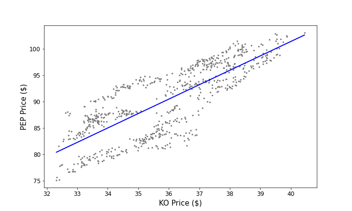
Linear relationship of the stock prices of Coca-cola and Pepsi
By purchasing one unit of Coca-cola and shorting $\beta$ units of Pepsi, we can construct a mean-reverting portfolio of the two stocks with mean equal to $\mu$. The portfolio value is $$ P = Y - \beta X = \Delta + \mu $$
Now, how can we construct a trading strategy around this mean-reverting portfolio? When the portfolio value deviates below the mean by some threshold, we should purchase the portfolio. We expect the portfolio value will increase as it returns to the mean. We can hold the portfolio until this happens and then close our position, taking a profit in the process. Likewise, when the portfolio deviates above the mean by some threshold, we should short the portfolio since we expect the portfolio value to decrease in the future.
The threshold by which we enter a position on the portfolio is typically some multiple of the standard deviation, $\sigma$, of the portfolio value in our training data. It is worth trying several values and finding what works the best according to the training data. A metric that is often used to judge a trading strategy is the Sharpe ratio, defined as $$ S = \frac{E[x] - E[r]}{\sigma} $$ where $E[x]$ is the expected return of our trading strategy, $E[r]$ is the expected risk-free rate, and $\sigma$ is the standard deviation of our returns. Typically, a smaller Sharpe ratio can indicate two potential things - smaller returns, or a higher variance of returns. Strategies with larger Sharpe ratios are therefore expected to yield greater returns, contain less risk, or both. For these reasons, strategies with higher Sharpe ratios are generally superior.
Here, we will impose that if the portfolio value deviates by $\pm 1.5 \sigma$ from the mean, we will take the appropriate position with our portfolio. When the portfolio value returns to within $0.5 \sigma$ of the mean, we will close our position. Below is the portfolio value over time, with the times that we buy and hold the portfolio highlighted in green, and the times where we short the portfolio highlighted in red. We see that this strategy is relatively long term and we can hold a position for months at a time.
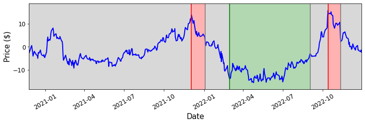
Statistical arbitrage strategy on our portfolio
How profitable is this strategy? Let's take a look at a chart of the profit, given that when we go long, we purchase one unit of the portfolio, and when we short, we short one unit of the portfolio.
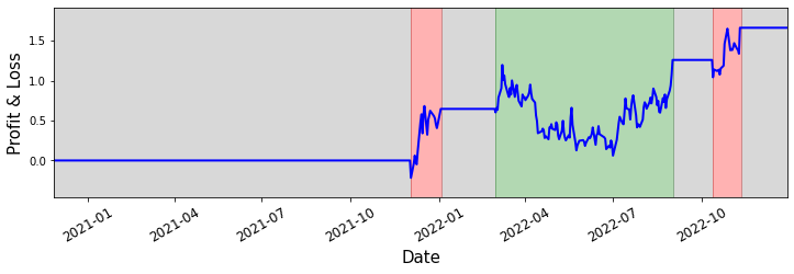
Profit / loss of our strategy
While this looks promising, what we have just done isn't exactly fair. We determined our trading strategy by calculating the mean and standard deviation of this data, and as a result calculating the profit of the training data is naturally biased towards being profitable. If we want to have some idea of how profitable this strategy is in practice, we need to try out this strategy on some future data. Consider some future data of the portfolio price, displayed below.
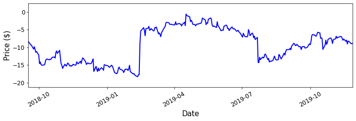
Portfolio value test data
If we implement the same trading strategy on this data, we go long or short at the following times and our profit curve is displayed below.
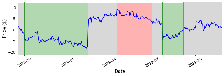
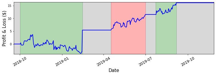
Portfolio strategy and PnL on test data
We find that the Sharpe ratio on the test data is $0.89$, which is okay but not great. Traditionally, a Sharpe ratio of 1 would be considered sufficient to implement a trading strategy. This leads us to an important point - as widespread algorithmic trading has increased the efficiency of markets, it has become more difficult to find excellent pair trading opportunities over time. Recall that by taking a position in our portfolio, we are purchasing an underperforming asset and shorting an overperforming asset. In doing this, we are pushing the price of the underperforming asset up, and pushing the price of the overperforming asset down. When many trading firms are executing a pair trading strategy simultaneously, the effect is that the prices deviate away from equilibrium less, reducing the standard deviation of the portfolio price and therefore reducing the profitability of each trade we make.
Clearly, we see that to profit substantially from this strategy we need to trade a significant number of units of the portfolio and bear a substantial amount of risk. In this example, we assumed that transaction costs are negligible. In practice, we must usually pay a fee to an exchange every time we buy or sell a stock. To more accurately determine the profitability of the strategy, we could include transaction costs in the calculation. We also assumed that we should only buy or sell a single unit of the portfolio in each trade. There are other ways to execute this trading strategy, such as by fully reinvesting the profit in every subsequent trade.
In general, it is worth maximising your exposure of the portfolio subject to risk constraints to maximise profit. As previously mentioned, one such risk constraint is to implement a stop-loss, such that if the portfolio deviates beyond what we expect, we close our position. As a result, we take a loss early before the loss becomes too great. We could also impose a maximum acceptable expected variance of our PnL, which will limit our potential returns but also make the returns more stable.
In this example we decided to enter a position on the portfolio when the portfolio value deviates more than $1.5 \sigma$ from the mean, closing the position when the portfolio value returns to within $0.5 \sigma$ of the mean. These thresholds determine the profitability of the strategy and are parameters that we are free to choose. A common technique that we could apply to this strategy is to consider a range of thresholds by which we enter and close our positions, choosing the parameters that maximise the Sharpe ratio for the training data.
To summarise, we see that there are many facets of the pair trading strategy that we can customise to maximise our profit and minimise our risk. Optimising a given strategy by considering these many possibilities is a core aspect of quantitative research.