Trading Analytics

In the following section, we will take public market data for BTC/USDT perpetual futures on Binance. This data is free and is accessible on their website here. We will calculate some common metrics for market data such as the market spread, and discuss approaches to calculate market volatility. Afterwards we will calculate common trading metrics such as the daily traded volume.

BBO Metrics

BBO metrics are metrics of best bid and offer (BBO) data. The offer is equivalent to the ask and can be used interchangeably. First, let's consider calculating the market spread over time. Recall that the spread is defined as $$ \text{spread} = \frac{p_{ \text{ask} } }{p_{ \text{bid} } } - 1. $$ The spread is typically described in basis points which as we saw in the trading course involves simply multiplying the spread by $10^4$.

bbo_data = pd.read_csv("btcusdt_bbo_data.csv").sort_values(by="transaction_time")
bbo_data["spread_bips"] = (bbo_data["best_ask_price"] / bbo_data["best_bid_price"] - 1) * 10**4

Likewise, to determine the market mid-price, we can simply code the definition of the mid-price, $$ p_{\text{mid}} = \frac{p_{\text{ask}} + p_{\text{bid}}}{2} $$ into pandas.

bbo_data["mid_price"] = (bbo_data["best_bid_price"] + bbo_data["best_ask_price"]) / 2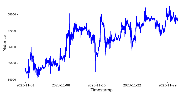

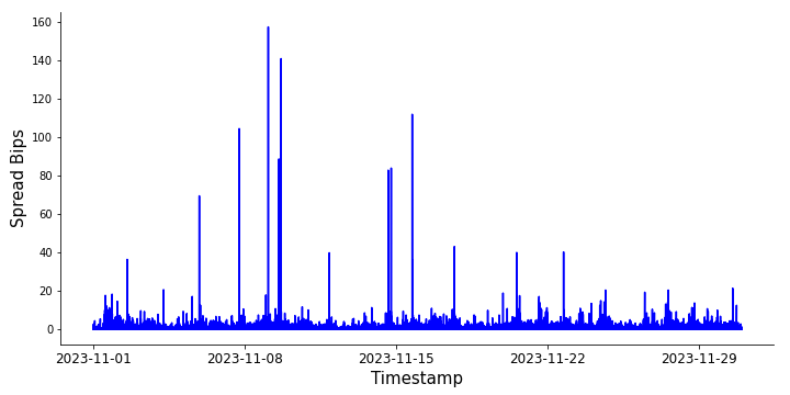
Midprice and spread of BTC/USDT perpetual futures

×

❮

❯

Aggregations - Sliding Window

A sliding window is a technique used to analyze a time series by considering consecutive windows of fixed length within that time series. The window 'slides' or moves across the data, one time step at a time, and at each step, operations are performed within the window. Suppose we want to calculate the volatility of an asset. A common method for calculating the volatility is to simply calculate the standard deviation of returns. However, we cannot calculate the standard deviation of a single value, and likewise calculating the standard deviation of the entire dataset does not give us much information - only a single data point. So, we calculate the volatility using a sliding window of some fixed size. There are two basic types of sliding window we could use;

• Update-based window: a sliding window over a fixed number of rows in the DataFrame.
• Time-based window: a sliding window over a fixed time interval in the DataFrame.

df[col].rolling(window=window_size)

where window_size is an integer corresponding to the number of rows the sliding window slides across. Now, let's implement a volatility calculation for ourselves.

def get_volatility_update_window(df: pd.DataFrame, window_size: int):
    if "mid_price" not in df.columns:
        df.loc[:, "mid_price"] = (df.loc[:, "best_bid_price"] + df.loc[:, "best_ask_price"]) / 2
    
    df.loc[:, "log_returns"] = df.loc[:, "mid_price"].pct_change().apply(lambda x: np.log(1 + x)) * (10 ** 4)
    
    df.loc[:, f"volatility_{window_size}"] = df.loc[:, "log_returns"].rolling(window=window_size).std().dropna()
    
    return df

bbo_data["transaction_time"] = pd.to_datetime(bbo_data["transaction_time"],unit='ms')

def get_volatility_time_window(df: pd.DataFrame, time_interval: str):
    if "mid_price" not in df.columns:
        df.loc[:, "mid_price"] = (df.loc[:, "best_bid_price"] + df.loc[:, "best_ask_price"]) / 2
    
    df.loc[:, "log_returns"] = df.loc[:, "mid_price"].pct_change().apply(lambda x: np.log(1 + x)) * (10 ** 4)
    
    df.loc[:, f"volatility_{time_interval}"] = df.loc[:, "log_returns"].rolling(window=time_interval).std().dropna()
    
    return df

Below we show two time-based sliding window calculations for the volatility. One has a sliding window length of 1000s and the other has a length of 10000s. Notice how increasing the size of the sliding window has the effect of smoothing the volatility over time. This is a useful property - volatility can be used as a trading signal, and smoothing the volatility over time can remove unwanted noise. Unwanted noise might come from large market orders which rapidly change the price for example. However, if the price recovers to it's initial state this price movement is not important to us, and we instead want to focus on volatility caused by changes in the market's view of the price of the asset.

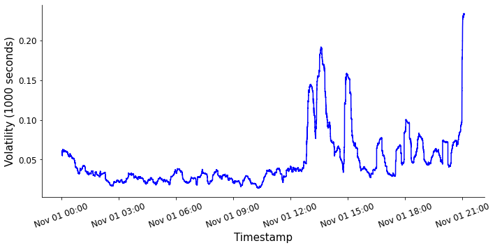
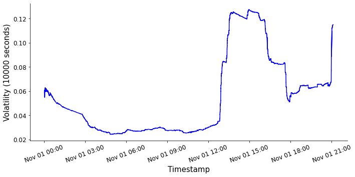
Volatility metric time-series

×

❮

❯

Aggregations - Groupby

The groupby functionality in pandas is extremely useful for quantitative research. In the following subsection, we will use groupby to obtain several important metrics.

Time-weighted average spread

Time-weighted average spread is an aggregated metric of the spread, where the spread at each time is weighted by the time for which the spread is maintained and averaged. It is defined as $$ \text{TWAS} = \frac{1}{T} \sum_{i=1}^N \text{spread}(t_i) \cdot \Delta t_i $$ where $T = \sum_{i=1}^N \Delta t_i$ is the total time within the aggregation time frequency, $\text{spread}(t_i)$ is the spread at time $t_i$ and $\Delta t_i = t_{i+1} - t_i$ is the duration of $t_i$. Let us now create some Python code that will calculate this for us.

The first thing to do is to get columns in our BBO data corresponding to the spread at each time $t_i$, and to $\Delta t_i$, the duration of each $t_i$. We already have some code to calculate the spread

bbo_data["spread_bips"] = (bbo_data["best_ask_price"] / bbo_data["best_bid_price"] - 1) * 10**4

and to calculate $\Delta t_i$ we simply need to take the difference of the timestamps between each consecutive row. Pandas has functionality built in for this, the .diff() method. When we calculate .diff() the first row will always be a NaN, since there is no row above it to calculate the difference. So, we replace this NaN with a zero using .fillna(0)

bbo_data["time_diff"] = bbo_data["transaction_time"].diff().dt.total_seconds().fillna(0)

Now, we have everything that we need to calculate the weighted spread, $\text{spread}(t_i) \cdot \Delta t_i$.

bbo_data["weighted_spread"] = bbo_data["spread_bips"] * bbo_data["time_diff"]

We can now perform the aggregation. To do this, we can use pandas' resampling functionality, which will automatically group by a time-frequency which we specify and return a pandas GroupBy object. We can then perform whatever operation we want on the time groupby object. Here we will calculate the minutely time-weighted average spread, which we can see here is denoted as "min".

grouped_by_time_freq = bbo_data.set_index("transaction_time").resample("H")

What remains is to simply sum the weighted spread column and the time_diff column, and take the ratio of the two. This give us our definition of the time-weighted average spread above.

weighted_spread_sum = grouped_by_time_freq['weighted_spread'].sum()
time_diff_sum = grouped_by_time_freq['time_diff'].sum()
time_weighted_average_spread = weighted_spread_sum / time_diff_sum

Let's compare plots of the spread and the minutely time-weighted average spread.

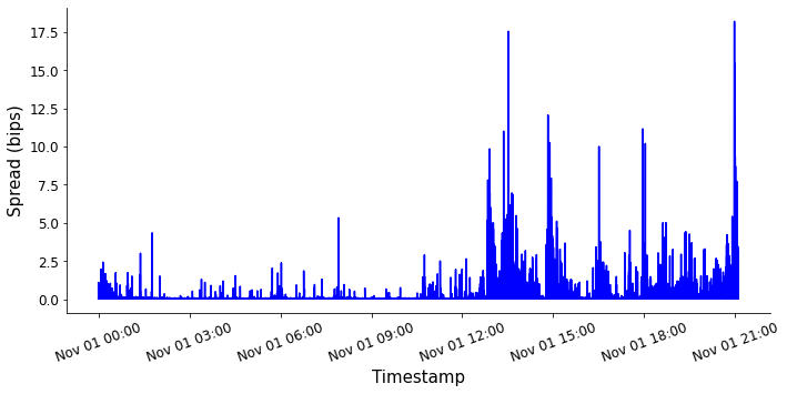
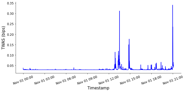
Spread and minutely TWAS

×

❮

❯

We see that aggregating the spread over time has a smoothing effect, similar to what we saw when we calculated the volatility. As before, this metric is useful because it filters out unwanted noise in the data.

Aggregated Traded Volume

The aggregated traded volume is a metric of the sum of the quantity of all trades within a specific time-frequency. This calculation is very straightforward to implement and highly useful in practically all trading firms. As a result, you should try it as an exercise. Trade data is also freely available on Binance and can be downloaded here.

trade_data = pd.read_csv("btcusdt_trade_data.csv").sort_values(by="time")

trade_data["time"] = pd.to_datetime(trade_data["time"], unit="ms")
trade_data = trade_data.set_index("time")

trade_data["volume"] = trade_data["price"] * trade_data["qty"]

def get_traded_volume(trade_data: pd.DataFrame, frequency: str) -> pd.Series:
    if not isinstance(trade_data.index, pd.DatetimeIndex):
        trade_data["time"] = pd.to_datetime(trade_data["time"], unit="ms")
        trade_data = trade_data.set_index("time")
    trade_data["volume"] = trade_data["price"] * trade_data["qty"]
    return trade_data["volume"].resample(frequency).sum()

Volume-weighted Average Price

Volume-weighted average price (VWAP) is a metric which tells us an average traded price, by weighting all trades by their volume. As a result, within a specific timeframe we can know what the average price was for a unit of the asset. Definition of the VWAP is $$ \text{VWAP} = \frac{1}{V} \sum_{i=1}^{N} v_i p_i $$ where there are $N$ trades within the timeframe, $v_i$ is the volume of the trade $i$, $p_i$ is the price per each unit traded within the trade $i$, $V = \sum_{i=1}^{N} v_i$ is the total traded volume within the timeframe.

trade_data["volume_x_price"] = trade_data["volume"] * trade_data["price"]

agg_volume = trade_data["volume"].resample(frequency).sum()
agg_volume_x_price = trade_data["volume_x_price"].resample(frequency).sum()

vwap = agg_volume_x_price / agg_volume

def calculate_vwap(trade_data: pd.DataFrame, frequency: str) -> pd.Series:
    if not isinstance(trade_data.index, pd.DatetimeIndex):
        trade_data["time"] = pd.to_datetime(trade_data["time"], unit="ms")
        trade_data = trade_data.set_index("time")
    trade_data["volume"] = trade_data["qty"] * trade_data["price"]
    trade_data["volume_x_price"] = trade_data["volume"] * trade_data["price"]
    agg_volume = trade_data["volume"].resample(frequency).sum()
    agg_volume_x_price = trade_data["volume_x_price"].resample(frequency).sum()
    vwap = agg_volume_x_price / agg_volume
    return vwap